Data preparation

Estimated time: 60 minutes

Overview

Questions

• Why do we divide data into training, validation, and test sets?
• What is data augmentation, and why is it useful for small datasets?
• How can random transformations help improve model performance?

Objectives

• Split the dataset into training, validation, and test sets.
• Prepare image and label arrays in the format expected by PyTorch.
• Apply basic image augmentation to increase training data diversity.
• Understand the role of data preprocessing in model generalization.

Partitioning the dataset

---

Before training our model, we must split the dataset into three subsets:

• Training set: Used to train the model.
• Validation set: Used to tune parameters and monitor for overfitting.
• Test set: Used for final performance evaluation.

This separation helps ensure that our model generalizes to new, unseen data.

To ensure reproducibility, we set a random_state, which controls the random number generator and guarantees the same split every time we run the code.

PyTorch expects image input in the format:

[batch_size, channels, height, width]

So we’ll also expand our image and label arrays to include the channel dimension at the start (grayscale images have 1 channel).

PYTHON

from sklearn.model_selection import train_test_split

# Reshape arrays to include a channel dimension:
# [height, width] → [1, height, width]
dataset_expanded = dataset[:, np.newaxis, :, :]
labels_expanded = labels[..., np.newaxis]

# Create training and test sets (85% train, 15% test)
dataset_train, dataset_test, labels_train, labels_test = train_test_split(
    dataset_expanded, labels_expanded, test_size=0.15, random_state=42)

# Further split training set to create validation set (15% of remaining data)
dataset_train, dataset_val, labels_train, labels_val = train_test_split(
    dataset_train, labels_train, test_size=0.15, random_state=42)

print("No. images, channels, x_dim, y_dim) (No. labels, 1)\n")
print(f"Train: {dataset_train.shape}, {labels_train.shape}")
print(f"Validation: {dataset_val.shape}, {labels_val.shape}")
print(f"Test: {dataset_test.shape}, {labels_test.shape}")

OUTPUT

No. images, channels, x_dim, y_dim) (No. labels, 1)

Train: (505, 1, 256, 256), (505, 1)
Validation: (90, 1, 256, 256), (90, 1)
Test: (105, 1, 256, 256), (105, 1)

Data Augmentation

---

Our dataset is small, which increases the risk of overfitting, when a model learns patterns specific to the training set but performs poorly on new data.

Data augmentation helps address this by creating modified versions of the training images on-the-fly using random transformations. This teaches the model to become more robust to variations it might encounter in real-world data.

We can use torchvision.transforms.v2 to define the types of augmentation to apply.

PYTHON

from torchvision.transforms import v2

# Define what kind of transformations we would like to apply
# such as rotation, crop, zoom, position shift, etc
datagen = v2.Compose([
    v2.RandomRotation(degrees=0),
    v2.RandomAffine(degrees=0, translate=(0, 0), scale=(1.0, 1.0)),
    v2.RandomHorizontalFlip(p=0.0)
])

Challenge

Exercise

1. Modify the datagen pipeline to include one or more of the following:

• v2.RandomRotation(degrees=20)
• v2.RandomResizedCrop(size=(256, 256), scale=(0.8, 1.0))
• v2.RandomHorizontalFlip(p=0.5)

Show me the solution

1. Here’s an example:

PYTHON

datagen = v2.Compose([
    v2.RandomRotation(degrees=20),
    v2.RandomResizedCrop(size=(256, 256), scale=(0.8, 1.0)),
    v2.RandomHorizontalFlip(p=0.5)
])

Now let’s view the effect on our X-rays!:

PYTHON

# specify path to source data
path = os.path.join("chest_xrays")
batch_size=5

# For visualization, we'll manually apply the transforms to a few images
import torch
from PIL import Image

def plot_images(images_arr):
    fig, axes = plt.subplots(1, 5, figsize=(20,20))
    axes = axes.flatten()
    for img, ax in zip(images_arr, axes):
        # Convert tensor back to numpy for plotting
        img_np = img.squeeze().numpy()
        ax.imshow(img_np, cmap='gray')
    plt.tight_layout()
    
sample_images = [Image.open(random.choice(effusion_list)).convert('L') for _ in range(batch_size)]
augmented_images = [datagen(torchvision.transforms.v2.functional.to_image(img)) for img in sample_images]
plot_images(augmented_images)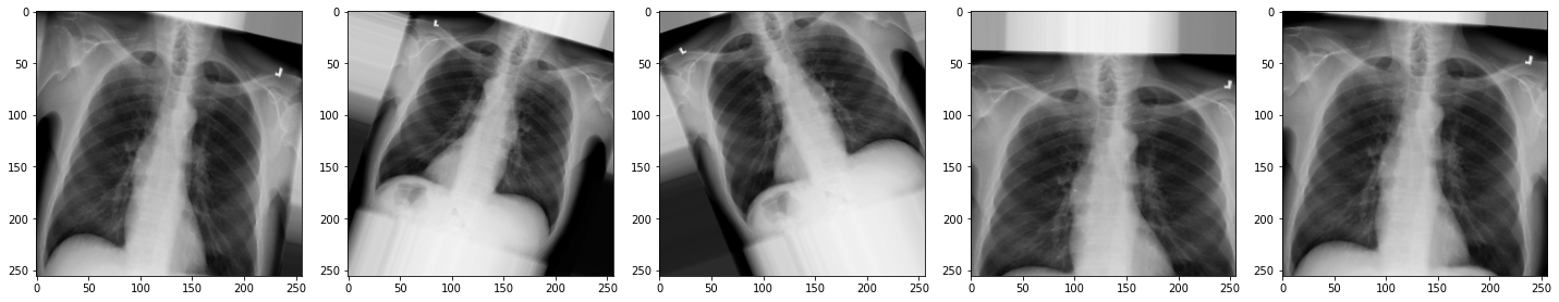

Challenge

Exercise

1. How do the new augmentations affect the appearance of the X-rays?
   Can you still tell they are chest X-rays?

Show me the solution

1. The augmented images may appear rotated, zoomed, or flipped.
   While they might look distorted, they remain visually recognizable as chest X-rays. These augmentations help the model generalize better to real-world variability.

In medical imaging, always consider clinical context. Some transformations, like left-right flipping, could lead to anatomically incorrect inputs if not handled carefully.

Now we have some data to work with, let’s start building our model.

Key Points

• Data should be split into separate sets for training, validation, and testing to fairly evaluate model performance.
• PyTorch expects input images in the shape (batch, channels, height, width).
• Data augmentation increases the variety of training data by applying random transformations.
• Augmented images help reduce overfitting and improve generalization to new data.